
Data Engineering Bootcamp Course Notes: Section 1 Dimensional Data Modelling
Notes from section 1 the Data Engineering Bootcamp, covering complex data types, OLTP vs. OLAP, cumulative tables, idempotent pipelines, SCDs, and more.

I’ve had the honour of working with lots of amazing Data Engineers and Analytics Engineers in my career.
So, when I saw that Zach Wilson was starting a course covering core Data Engineering concepts I decided to give it a go, with the goal of refining my Data Engineering skills and filling in any knowledge gaps.
If you are interested in taking the course it can be found at https://bootcamp.techcreator.io/
Each week I will share a post with my key learnings from the course.
Quick note: The course assumes a foundational understanding of data concepts. If these notes feel too high level, stay tuned for future posts where I’ll explore some of these topics in greater depth.
Complex Data Types
You probably know the standard data types; STRING, INT, REAL, BOOLEAN.
Many modern databases also support complex data types, which unlock new possibilities for data modeling.
Struct: Key, Value pairs. Where the keys are rigidly defined.
Compression: Good
Values: Any type
Map: Keys loosely defined. E.g. a place where you can store different data for each row.
Compression: Okay
Values: Always the same type
Array: Ordinal list
Values: Always the same type - but they can be maps or structs!
Data Modelling
Effective data modeling begins with understanding the needs of your end users
Data engineers: data types that compress data effectively, don’t worry about complexity
Analytics teams: data types that are easy to use - limit arrays, structs and maps.
ML model: tailor for the model, usually this means a flat table.
OLTP vs Master Data vs OLAP
OLTP: Online Transaction Processing: Optimised for low latency, low volume queries. This usually means one user at a time.
For example, think of Amazon showing you your most recent order, they don’t need to look at anyone else's data to do that.
OLTP data is usually normalized, which is often best for this, e.g. 3rd normal form.Master data: Complete definitions. Data deduplicated. Used as a condensed version of OLTP data before transforming into OLAP data.
OLAP: Online Analytical Processing: Optimised for large volume queries. Using group bys but minimising joins.
For example, if Amazon wanted to calculate total sales today they’d need the data from every customer to do that.Think of these as a continuum changing the data to suit its use case and end users
Production Database Snapshots (OLTP) -> Master Data -> OLAP -> Metrics
Compactness vs Usability tradeoff
Most compact tables - aren’t human readable
They are compressed to be as small as possible.
Common for OLTP
Use for online applications where latency and data volumes matter a lot. Users are usually highly technical (e.g. software engineers) who are building software to process the output.
Middle ground tables
Use complex data types (e.g. arrays, structs and maps) to compact data.
Common for Master data
Use for upstream staging or master data where most users are data engineers.
Most Usable
No complex data types (e.g. arrays, structs and maps)
Can be easily manipulated using WHERE and GROUP BY
Common for OLAP
Use for analytics tables.
The Case for Complex Data Types
Imagine you are looking at AirBnB data
6 million properties.
Availability for the next year - 365 nights
This results in 2 billion pairs of properties and nights (6 million × 365).
What’s the best way to store this data?
Listing level with an array of nights - 6 million rows
Listing night level - 2 billion rows
When properly sorted, Parquet can compress this data efficiently using run-length encoding.1
But when it queries spark shuffles the data, if this happens to you your file size will explode. And you can’t stop people querying the data.
Cumulative Table Design
This approach is an effective method for creating tables that combine historical data with current records
For example at Meta it is used to track user data, by looking at a single day of data you can see when a user was last active.
How to
Join yesterday's cumulative table with today's new data.
Full outer join the two data frames together: this ensures you get all relevant rows. If we look at user data this would ensure we get users who are new today (only in today’s table) and users who were active in the past but not today (only in yesterday’s table).
Coalesce the values to deal with nulls
Keep the history
Interestingly, a variation of this approach was part of an interview question I encountered during my time applying to Facebook in 2017.
Advantages
Seamless integration of historical data for analysis.
Queries are often simpler than doing historical analysis from scratch
Easy to do transition analysis - for example finding when a user went from active to churned.
Drawbacks
Can only be backfilled sequentially - so can’t be parallelised. This can make backfilling a lot of history really really slow.
Handling PII data can be challenging as deleted users get carried forward unless there is separate code to prevent this.
How to code a cumulative table
Example Code provided by Zach.
Idempotency
Idempotency is crucial. It is the idea that data pipelines run on the same data should produce the same output. Regardless of which day you run it, what time you run it or how many times you run it.
Without idempotency, pipelines become challenging to debug and reason about effectively. You will get silent failures. Unit tests will no longer be a reliable indicator of pipeline quality. Data won’t be consistent.
Common reasons a pipeline isn’t idempotent
INSERT INTO without TRUNCATE: Each time you run the pipeline new data will get added. Use MERGE or INSERT OVERWRITE instead.
Start data without an end date: If you run it tomorrow you get an extra row of data that you didn’t get today.
Not using a full set of partition sensors: Inserting data when the source data isn’t fully loaded. Then if you run it again later when the data is fully loaded it will give different results.
Not using depends_on_past for cumulative tables. So if yesterday's data is missing you lose the full history.
Using the latest partition rather than the correct one for the day you are looking at.
SCD: Slowly Changing Dimensions
Dimensions provide context and background information about your data.
For example you might have a “dim” (dimension) table of customers that includes their name, address and registration date.
Some dimensions don’t change
For example: Registration date, date of birth, height
Some dimensions do change
For example: Address - which changes every time you move house
These are slowly changing dimensions.
SCD Modelling Options
Type 0 Never changes: Used for unchanging dimensions.
Type 1 Latest snapshot: Keep only the most recent row.
Use if you only care about the most recent value.
Don’t use it as it makes pipelines not idempotent.
Type 2 Full history: You care about what the values were and when they were these values.
Best type of SCD
Type 3 Original and current value
Lose history between original and current.
Like type 0, don’t use it as it makes pipelines not idempotent.
How to store Type 2 data
Type 2 can be stored in two main ways
Daily snapshot: Keep one row per day
Simple to use and work with
Space inefficient
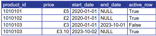
Value and Applicable Dates: Track the value and its applicable dates
Current values have an end date that is NULL or far into the future 9999-12-31
More than one row per dimension so requires care when joining. The start and end dates must always be used. Can be simplified with a current_row boolean.
How to transform the data into a value and dates structure
Entire history in one query:
This uses a method similar to my query for creating session IDs in my Advanced Data talk - slide 52 onwards.
Incrementally: Load one day at a time.
Additive and Non Additive Dimensions
Dimensions are Additive over a period of time if they can take exactly one value in that time.
Examples
Phone type per day is not additive as some people have both an iPhone and an Android phone.
Age per day is additive as each person is exactly one age.
In other contexts this is sometimes referred to as MECE: Mutually Exclusive and Collectively Exhaustive
Mutually Exclusive: no item has two values
Collectively exhaustive: every item has at least one value.
The benefit of additive dimensions is
You can sum them - Total population = population 0-50 + population 51+
You can use count(1) and get the correct totals, rather than needing count distinct
Note: often sum metrics work even for non additive dimensions.
For example:
Total users != Android users + iPhone users
But Total time spent = Android time spent + iPhone time spent
When should you use Enums
Enums are data types that can only contain a set of pre-specified named values.
Low to medium cardinality values. Generally up to about 50 distinct values.
Why should you use them
Built in data quality: will fail pipeline if you try to input the wrong value
Built in static fields: can bring in efficiently as they are part of the code
For example, a value, a cost or a benefit. Pulled directly from the ENUM list.
Built in documentation: people know all possible values, making the data easier to use.
Can be used for partitions: you know all the values they can be so you know you’ve covered everything.
Partitioning on date and enum can be good for large datasets.
One use case where they can be valuable is if you are ingesting data from a number of sources, you want to ingest differently for each one but also check all sources have landed. Zach has some code - https://github.com/EcZachly/little-book-of-pipelines which creates a reusable book of pipelines to use in both places.
Graph Modelling
Most data is modelled via tables, but sometimes you are most interested in the relationships between entities. In these cases graph modelling can be valuable.
Example graph
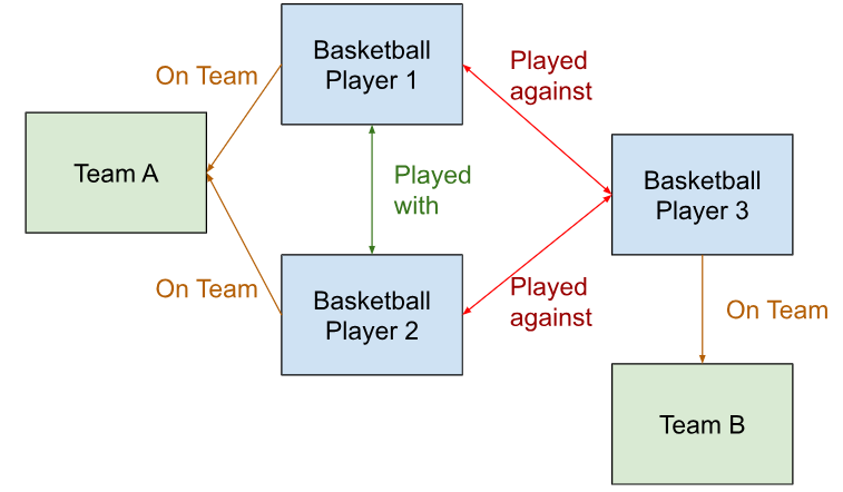
Here we have 2 kinds of Nodes
Players (1,2,3) in blue
Teams (A,B) in green
And 3 kinds of edges
On Team (in orange) - which team a player plays for
Played with (in dark green) - showing which team mates they’ve played games with
Played against (in red) - showing which other players they’ve played games against.
Data model for graph data
Entities or Nodes
Identifier: STRING
Type: STRING
Properties: MAP<STRING, STRING>
Relationships
Subject_identifier: STRING
Subject_type: VERTEX_TYPE
Object_identifier: STRING
Object_type: VERTEX_TYPE
Edge_type: EDGE_TYPE
Properties: MAP<STRING, STRING>
Conclusion
This post has explored foundational concepts of dimensional modelling, from understanding complex data types and their trade-offs to designing tables for various use cases, including OLTP, OLAP, and cumulative data. We’ve examined the importance of idempotency in pipeline design, strategies for managing Slowly Changing Dimensions, and considerations for modeling additive dimensions and graph data.
If you found these insights valuable I encourage you to explore Zach Wilson's course to deepen your understanding. Find it at https://bootcamp.techcreator.io/
Stay tuned for upcoming posts covering topics from the rest of the course.
I’d love to hear your thoughts—how do you tackle these challenges in your work? Share your experiences in the comments.
For an explanation of what this is see https://api.video/what-is/run-length-encoding/